LANDSAT Color Image Mapping
Introduction
So, continuing on from the last post, the next step is to construct color images, and map them.
LANDSAT has three bands, that when combined, can be used to create a color image. For more information on LANDSAT bands, look at https://www.mapbox.com/blog/putting-landsat-8-bands-to-work/.
Sadly the default color images that result don't have much of the 'wow!' factor, and they are usually very dark. There is a lot of material on how to add 'wow!' to LANDSAT images: for example see https://www.mapbox.com/blog/processing-landsat-8/. This usually involves handcraft Red/ Green/ Blue histogram changes, to bring out more details.
I will use the SciKit image processing tools to add 'wow!' to my map.
LANDSAT Color Bands
First we read in the three bands that will make up our color image.
    #  enable gdal exceptions (instead of the silent failure which is gdal default)
    gdal.UseExceptions()

    # Bands 2, 3, and 4 are visible blue, green, and red.

    fname_red = '../data/LC80890792016366LGN00_B4.tif'
    fname_blu = '../data/LC80890792016366LGN00_B2.tif'
    fname_grn = '../data/LC80890792016366LGN00_B3.tif'

    ds_red = gdal.Open(fname_red)
    ds_blu = gdal.Open(fname_blu)
    ds_grn = gdal.Open(fname_grn)

    data_red = ds_red.ReadAsArray()
    data_grn = ds_grn.ReadAsArray()
    data_blu = ds_blu.ReadAsArray()
Then we create a numpy array to hold all three color planes (I should really check that
all three planes have the same size, but in this case I trust NASA)
    rgb_size = 3

    data_rgb = np.zeros((ds_red.RasterYSize, ds_red.RasterXSize, rgb_size ))
Scaling for image processing
The SciKit image processing utilities seem to insist that pixel values be scaled between -1 to + 1. We scale our pixel value accordingly.
    r = np.max(data_red)
    g = np.max(data_grn)
    b = np.max(data_blu)


    data_rgb[:,:,0] = data_red/max(r, b, g)
    data_rgb[:,:,1] = data_grn/max(r, b, g)
    data_rgb[:,:,2] = data_blu/max(r, b, g)

    data_one = np.ones((ds_red.RasterYSize, ds_red.RasterXSize, 3))

    # clip all pixel value to 1.0
    data_rgb = np.minimum(data_rgb, data_one)
Mapping the raw color image
So at this stage we have our color image contained in the variable data_rgb. We execute the same logic as in the previous post
in this series; create projections for the image, map, and overlayed data, create an Axes object
with the same extent as the image (so all the image is displayed), add the image to the map, add overlayed data (coastlines, location of home),
and add gridlines, titles, etc.
    #  size in lon/lat of zoomed in  map area for subsequent plots
    x0 = 153.03
    x1 = 153.12
    y0 = -26.605
    y1 = -26.515

    # set up projection constants

    zone = 56
    projection = ccrs.UTM(zone, southern_hemisphere=False)

    img_CRS = projection

    plot_CRS = ccrs.PlateCarree()
    geodetic_CRS = ccrs.Geodetic()


    # transform limits of plot to zoomed in map projection units
    x0, y0 = plot_CRS.transform_point(x0, y0, geodetic_CRS)
    x1, y1 = plot_CRS.transform_point(x1, y1, geodetic_CRS)

    # create figure and axes
    plt.figure(figsize=(12,8), dpi=100)
    ax = plt.axes([0,0,1,1], projection=plot_CRS)

    extent_tif = (gt[0], gt[0] + ds.RasterXSize * gt[1],
              gt[3] + ds.RasterYSize * gt[5], gt[3])

    # get tif limits in map coordinates
    tx0, ty0 = plot_CRS.transform_point(extent_tif[0], extent_tif[2], img_CRS)
    tx1, ty1 = plot_CRS.transform_point(extent_tif[1], extent_tif[3], img_CRS)

    # show whole image
    extent_map = (tx0, tx1, ty0, ty1)


    ax.set_extent(extent_map, plot_CRS)

    img = ax.imshow(data_rgb, extent=extent_tif,transform = img_CRS,
                    origin='upper',)

    ax.coastlines(resolution='10m',zorder=4, color='navy')
    gl = ax.gridlines( draw_labels=True)

    # suppress gridline labels at top to allow space for title
    gl.xlabels_top = False

    # example overlay of lat/lon data
    ax.plot(153.09, -26.53, marker='o', markersize=10, color='red', transform=ccrs.Geodetic())

    ax.set_title('LANDSAT Band 432 (True Color),\nLANDSAT_SCENE_ID = LC80890792016366LGN00')

    plt.show()
This gives us the following map:
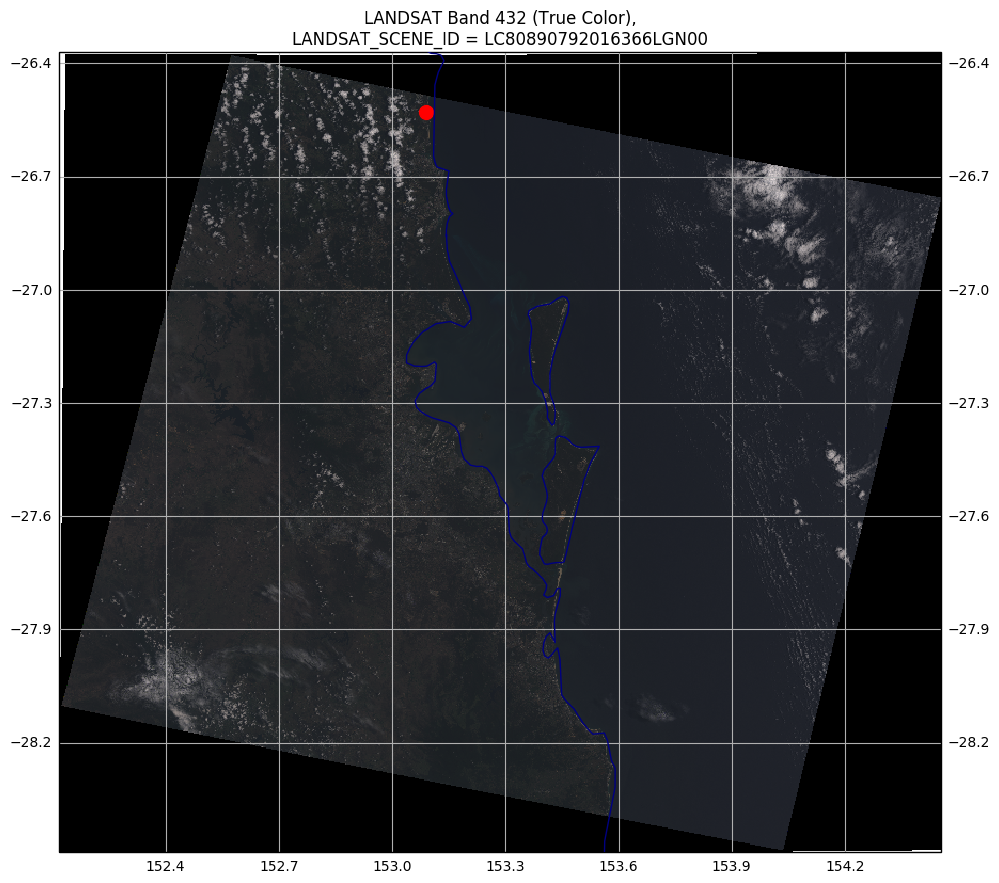
The image appears very dark, because NASA scales images to accomodate very bright saltpans, snow, etc.
Adjusting the image
I used the SciKit Image Exposure tools to investigate the best way to add 'wow!'. First I tried adjusting the Gamma (effectively performing nonlinear scaling to make dark pixels brighter), but I was not overly impressed. High values of scaling seemed to wash out the image. In all, I tried
-
Gamma Adjustment
-
Sigmoidal Adjustment
-
Logarithmic Adjustment
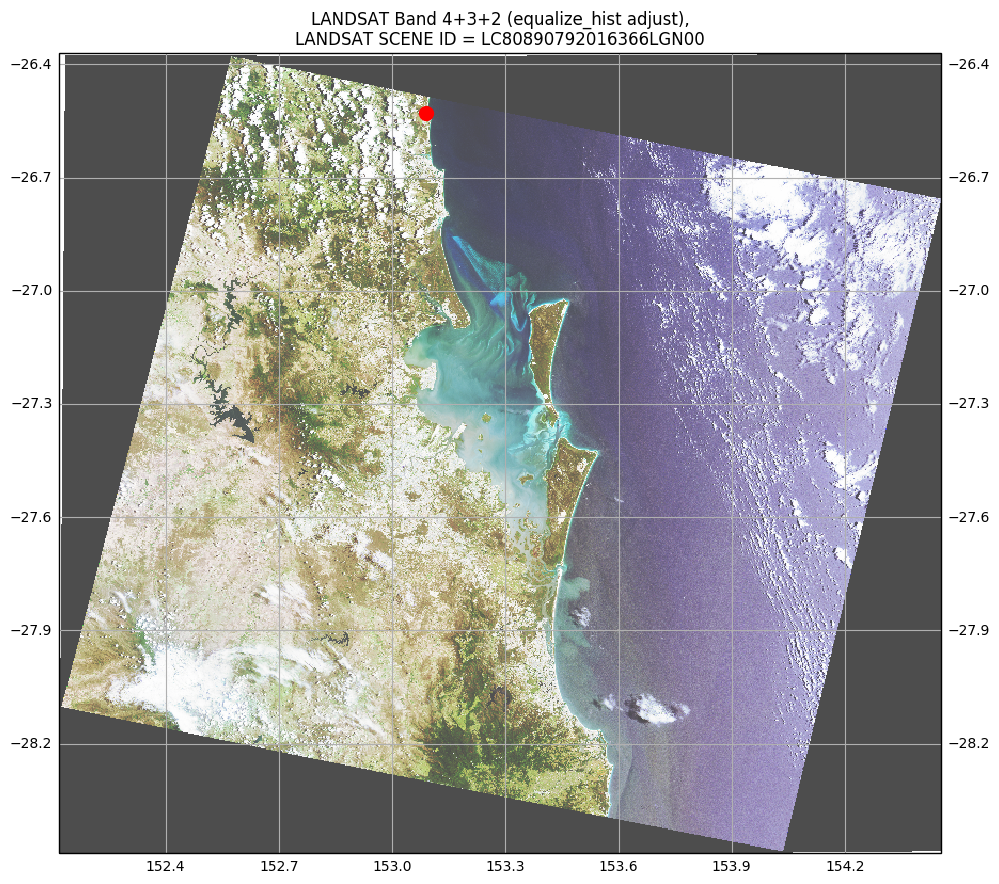
Finally I settled on individual color plane histogram adjustment.
    eq_red = skimage.exposure.equalize_hist(data_red)
    eq_blu = skimage.exposure.equalize_hist(data_blu)
    eq_grn = skimage.exposure.equalize_hist(data_grn)

    r = np.max(eq_red)
    g = np.max(eq_grn)
    b = np.max(eq_blu)

    eqh = np.zeros((ds_red.RasterYSize, ds_red.RasterXSize, rgb_size ))

    eqh[:,:,0] = eq_red/max(r,g,b)
    eqh[:,:,1] = eq_grn/max(r,g,b)
    eqh[:,:,2] = eq_blu/max(r,g,b)
followed by the same code as before, with the image display call being:
    img = ax.imshow(eqh, extent=extent_tif, transform = img_CRS,
                    origin='upper',)
This gives us:
Conclusion
I have new-found respect for the science and art of processing LANDSAT images in order to convey information to humans (as opposed, say, to automated vegetation habitat classification).
Just for completeness, here are the imports for all the code above (and some code to come) (some are used only to support print-outs that define the environment for reproducibility purposes) :
    # all imports should go here

    import pandas as pd

    # most of these following are used to support repeatability of the notebook
    import sys
    import os
    import subprocess
    import datetime
    import platform
    import datetime
    import math

    import matplotlib.pyplot as plt

    # support for TIFF input
    import gdal
    import osr

    import cartopy.crs as ccrs
    import cartopy

    import numpy as np

    # used for color image processing
    import skimage.exposure
    import skimage.io as sio
The notebook that has all the code is coming soon.
Comment